Advanced Excel tips

Had user who need to freeze top row of Excel sheet:

Freeze Versus Lock in Excel

As we briefly mentioned above, if you want a row or column to be visible no matter where you scroll in your Excel sheet, this requires the freeze feature.
You would use the lock feature to prevent changes to the content of a cell. As examples, you might lock a cell or range that contains formulas, lists, or similar types of data that you don’t want changed.
So if someone asks you how to lock a row in Excel, they likely mean to ask how to freeze a row in Excel.

How to Freeze the First Column or Top Row in Excel

More spreadsheets than not contain column or row headers. So freezing a column or row containing headers make is much easier to manage your data, especially when you have a lot of it.
With this method, you’re going to have to choose to freeze either the first column or first row. Unfortunately, you can’t do both.

1. Open your Excel spreadsheet and go to the View tab.
2. Click the Freeze Panes button.
3. To freeze the first column, click Freeze First Column in the dropdown menu. To freeze the top row, click Freeze Top Row.

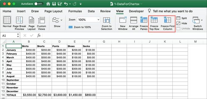
In Excel on Mac, you have separate buttons on the View tab for each option. So just click Freeze First Column or Freeze Top Row.

How to Freeze Columns and Rows in Excel

You may want to freeze more than just the first column or row in Excel. For instance, maybe you want to freeze the first three columns or rows.

1. Open your Excel spreadsheet and go to the View tab.
2. Select the last column or row in the group you want to freeze. For example, if you want to freeze columns A through C, select column D. Or if you want to freeze rows 1 through 4, select row 5.
3. Click the Freeze Panes button and then the Freeze Panes option in the dropdown menu.

In Excel on Mac, this is also its own button on the View tab. So select the column or row and click Freeze Panes.

How to Freeze Panes in Excel

If you would prefer to freeze a combination of rows and columns, referred to as a pane, it’s possible but slightly trickier.

1. Open your Excel spreadsheet and go to the View tab.
2. Select the cell directly below the row you want to freeze and the cell to the right of the column you want to freeze. For example, if you want to freeze columns A through C and rows 1 to 4, you would select cell D5.
3. Click the Freeze Panes button and again, click the Freeze Panes option in the dropdown menu.

How to Unfreeze Columns, Rows, or Panes in Excel

It’s just as simple to unfreeze columns, rows, and panes in Excel as it is to freeze them.

1. Open your Excel spreadsheet and go to the View tab.
2. Click the Freeze Panes button.
3. Select Unfreeze Panes in the dropdown menu.

In Excel on Mac, as you may have already guessed, this too is its own button. Head to the View tab and click Unfreeze Panes.




From https://www.makeuseof.com/